Greetings everyone,
I ran the Urban Flood Risk Mitigation model for a province located in Vietnam (see LULC below)
Here, the green/brown areas are vegetation, the red ones are urban areas and the blue is water.
I wonder why I got this result (see next image), where the areas where water is located have the highest values (very high), while where there’s vegetation, the runoff retention is low (is runoff retention the ability of soil to absorb water?). Given this image, if it’s correct, where would you say the risk of flooding is higher?
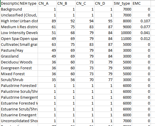
I attach the biophysical table that I used to run this model. More information on my land use classes here http://maps.elie.ucl.ac.be/CCI/viewer/download/ESACCI-LC-QuickUserGuide-LC-Maps_v2-0-7.pdfBiophysical_water.csv (761 Bytes)
Thank you for your help,
Marco
Besides, looking at the Biophysical table of the InVEST Sample Data, I wonder what “SW_type” and “EMC” mean.

Thank you,
Marco
1 Like
Hello Marco,
I may have at least partial answers for you.
First, runoff retention, as you mention, is the amount of water absorbed by soil and vegetation, so the fact that you have zero retention on the vegetated land cover classes suggests a problem. My guess, looking at your biophysical table, is that the table is missing some entries for some of the intermediate vegetation cover classes (e.g. LULC #12, 62, 71, 72, 81, 82, 122, etc.). These appear to be present in your map but not in the table. I am not sure what happens when the model goes to look up a lucode in the table and doesn’t find it, but that might explain the 0 retention volume for those cover classes. For these intermediate cover classes, you could give them slightly lower curve number (CN) values than their ‘open’ cover equivalents (e.g. LULC #60, 70, 80, 120) to reflect the greater tree cover, or give them the same number as their respective open classes for now.
Second, in the example biophysical table as well as in yours, the ‘water’ and ‘wetland’ classes are given a curve number value of 1.0, which corresponds to a case of no retention in the SCS Method used by the model. I think this was an arbitrary choice to make open water show up in the output maps as places of localized flooding, but the CN could be changed to 0 (complete retention) if you are more interested in understanding the land’s retention capacity. However, this doesn’t explain why your ‘water’ cover classes have the highest (non-zero) retention in your output map. These pixels should have 0 retention, based on your biophysical table, so I am unsure what’s going on there…
Lastly, if you need a reference on the SCS Curve Number method (I don’t know if it’s included in the User’s Guide or not):
Hopefully your issues will be resolved by adding entries for the other land cover classes.
Regards,
Ben
1 Like
“SW_Type” was a parameter internal to the example development, and is not needed for the model. Not sure why it’s included in that table. “EMC” is the event mean concentration of a pollutant in mg/L; in this case the numbers look like Phosphorus to me, but I am unsure. It would be needed for a later step in the model to determine nutrient or pollutant retention associated with retained stormwater runoff.
1 Like


