Analyzing Spatio-Temporal Drivers of Water Yield Using InVEST SWY and Machine Learning – Need Feedback on Factor Selection

Hi everyone,

I’m currently working on a research project titled “Implementation of the InVEST model to assess seasonal and annual water yield in the Chambal and Subarnarekha River basins for improved water resource management.”

:magnifying_glass_tilted_left: One of the key objectives of my study is:

To identify the factors that influence changes in water yield over time and space.

To achieve this, I used the InVEST Seasonal Water Yield model for a 20-year time span (2002–2022) at 5-year intervals. I then applied a Random Forest-based feature importance analysis to generate a heatmap showing the relative influence of various biophysical and climatic factors over time.

:bar_chart: Current input factors used:

  • Precipitation (monthly/annual)
  • Reference Evapotranspiration (ET₀)
  • Slope
  • LULC (Land Use Land Cover)
  • Curve Number (CN)
  • Kc values (crop coefficients)

I would really appreciate community feedback on:

  • Is this selection of input factors sufficient and appropriate for understanding water yield variability?
  • Should I consider including or excluding any factors (e.g., soil texture, root depth, NDVI, soil moisture, etc.)?
  • Are there best practices for validating machine learning results in the context of InVEST outputs?

I’m attaching a sample of the heatmap I generated for reference

Looking forward to your valuable suggestions!

Best regards,
Swarnajit Roy
Symbiosis Institute of Geoinformatics

1 Like

@swolny guide me please

Hi @abir -

I have not worked with Random Forest specifically, but it sounds like you’re doing a sensitivity analysis to determine which factors have the greatest influence on model results. I like the heatmap you generated, it’s a nice way of visualizing.

When we do sensitivity analysis for InVEST models, we only use factors that are actual inputs to the models. So that includes Precipitation, ET0, LULC, CN and Kc, as you listed. Slope is not an explicit factor in SWY, so would not include it. Similarly, root depth, NDVI and others are not part of the model, so I would not include those. The model does include parameters alpha, beta and gamma, which we usually include in sensitivity analysis (see this Hamel et al 2020 paper for an example of this).

And I don’t have any advice about machine learning results, so will leave that to others who do have experience.

~ Stacie

@swolny @megannissel

I’m currently validating my Seasonal Water Yield model output (QF) using TerraClimate surface runoff (q) data as a proxy for ground truth. However, during the RMSE calculation between the model’s output (QF) and the TerraClimate data, I’m getting unusually high RMSE values (close to 100 mm). I’ve ensured both rasters are aligned and reprojected properly, and units have been converted appropriately.

Despite this, the values differ significantly. For instance, InVEST outputs much higher surface runoff than TerraClimate in most areas. I’m unsure whether:

  • This discrepancy is expected due to conceptual differences between QF and q in TerraClimate,
  • Or if there’s a preprocessing issue (e.g., rescaling, unit mismatch, nodata handling, etc.).

Has anyone faced similar issues during model validation? If so, I would greatly appreciate any insights on how to improve the accuracy or interpret these differences meaningfully.

Thanks in advance!

— Swarnajit Roy

@swolny @megannissel please reply

Hello @abir -

I have never used TerraClimate, so I just took a quick look at their methods. There seem to be some similarities with SWY, as well as a lot of differences. One big difference is that it explicitly includes snowpack, which SWY does not. It also looks like TerraClimate’s runoff includes some of the evapotranspiration processes that SWY uses to calculate local recharge and baseflow, where the quickflow result of SWY is mainly based on curve number, it does not include evapotranspiration or related processes, so it is much simpler.

What are you using as the precipitation and ET0 data for your SWY model? TerraClimate says they use WorldClim for precipitation and a modified Penman Montieth ET0 calculation, so there can also be significant differences in the initial precipitation and evapotranspiration values between your inputs and theirs, along with the differences in modeling methods.

When I’ve worked on studies where we compare our model output to a different model’s output, we have focused on how the patterns of high and low values compare, not the absolute values. If we have actual observed real-world data, then we focus more on the absolute values, and do sensitivity analysis and calibration to bring the model’s output closer to reality.

~ Stacie

1 Like

Hello @swolny

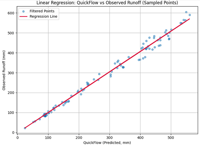
I am writing to share the results of the validation performed on our machine learning-based precipitation estimation using the WorldClim dataset for the year 2022. To ensure model reliability, a tolerance level was applied to address potential issues of overfitting and underfitting during training.

The validation results are as follows:

  • Root Mean Square Error (RMSE): 18.02 mm
  • Percentage RMSE Error: 6.26%
  • R² Score: 0.9878

These results indicate a high level of model accuracy and robustness. The validation plot for 2022 is attached for your reference.

Please let me know if further details or clarification are required.

CODE FOR VALIDATION

import rasterio

import numpy as np

from sklearn.linear_model import LinearRegression

from sklearn.metrics import mean_squared_error, r2_score

import xarray as xr

from rasterio.warp import reproject, Resampling

from rasterio.transform import from_bounds

import warnings

warnings.filterwarnings("ignore", category=FutureWarning)

# === Step 1: File Paths ===

qf_path = "/content/QF.tif"

terra_path = "/content/TerraClimate_q_2022.nc"

# === Step 2: Load QuickFlow TIFF ===

with rasterio.open(qf_path) as src_qf:

qf = src_qf.read(1)

qf_meta = src_qf.meta.copy()

qf = np.where(qf == src_qf.nodata, np.nan, qf)

# === Step 3: Load TerraClimate runoff and compute annual runoff ===

ds = xr.open_dataset(terra_path)

obs_data = ds['q'].sum(dim='time') # Annual runoff

obs_vals = obs_data.values

# === Step 4: Build Transform for Observed Data ===

lat = ds['lat'].values

lon = ds['lon'].values

height, width = len(lat), len(lon)

transform_obs = from_bounds(lon.min(), lat.min(), lon.max(), lat.max(), width, height)

# === Step 5: Reproject TerraClimate to Match QF ===

obs_resampled = np.empty_like(qf)

reproject(

source=obs_vals,

destination=obs_resampled,

src_transform=transform_obs,

src_crs="EPSG:4326",

dst_transform=qf_meta['transform'],

dst_crs=qf_meta['crs'],

resampling=Resampling.bilinear

)

obs_resampled = np.where(obs_resampled == 0, np.nan, obs_resampled)

# === Step 6: Flatten and Clean ===

qf_flat = qf.flatten()

obs_flat = obs_resampled.flatten()

mask = (~np.isnan(qf_flat)) & (~np.isnan(obs_flat))

qf_clean = qf_flat[mask]

obs_clean = obs_flat[mask]

# === ✅ Step 7: Apply Relative Error Tolerance (10% of individual observed values) ===

rel_tol = 0.10 # 10% relative tolerance

mask_tol = (np.abs(qf_clean - obs_clean) <= rel_tol * obs_clean)

X = qf_clean[mask_tol].reshape(-1, 1)

y = obs_clean[mask_tol]

if len(X) == 0:

raise ValueError("No points passed the relative error tolerance filter.")

# === Step 8: Train Linear Regression ===

model = LinearRegression()

model.fit(X, y)

y_pred = model.predict(X)

# === Step 9: Evaluation ===

rmse = np.sqrt(mean_squared_error(y, y_pred))

r2 = r2_score(y, y_pred)

mean_obs = y.mean()

rmse_percent = (rmse / mean_obs) * 100

# === Step 10: Print Results ===

print(f"Tolerance applied: ±10% of each observed value")

print(f"Points used in regression: {len(X)} / {len(qf_clean)} ({(len(X)/len(qf_clean))*100:.2f}%)")

print(f"Mean of Observed Runoff = {mean_obs:.2f} mm")

print(f"RMSE = {rmse:.2f} mm")

print(f"Percentage RMSE Error = {rmse_percent:.2f}%")

print(f"R² Score = {r2:.4f}")

import matplotlib.pyplot as plt

# === Limit to 100 random samples for visualization ===
np.random.seed(42)  # For reproducibility
if len(X) > 100:
    indices = np.random.choice(len(X), 100, replace=False)
    X_vis = X[indices]
    y_vis = y[indices]
    y_pred_vis = y_pred[indices]
else:
    X_vis = X
    y_vis = y
    y_pred_vis = y_pred

# === Plot ===
plt.figure(figsize=(8,6))
plt.scatter(X_vis, y_vis, alpha=0.5, s=30, label='Filtered Points')
plt.plot(X_vis, y_pred_vis, color='crimson', linewidth=2, label='Regression Line')
plt.xlabel("QuickFlow (Predicted, mm)")
plt.ylabel("Observed Runoff (mm)")
plt.title("Linear Regression: QuickFlow vs Observed Runoff (Sampled Points)")
plt.legend()
plt.grid(True)
plt.tight_layout()
plt.show()

@swolny just need you valuable insight :slightly_smiling_face: please response the last massage.

THANK YOU

This is cool @abir !

I’m not an expert with hydrological modeling, but I’m wondering about this step:

Are you filtering the data to only compare predicted values that are already within 10% of the observed value at that location? What’s the relationship like with no filtering applied?

1 Like

Hello @dave
Yes, the data is filtered to include only those points where the predicted QuickFlow value is within ±10% of the observed runoff at each location. This is done in the following line:

python

CopyEdit

mask_tol = (np.abs(qf_clean - obs_clean) <= rel_tol * obs_clean)

This ensures that the regression model is trained and evaluated only on points where the prediction error is relatively low.

is this incorrect ?

just let me know

I don’t know. I assumed your objective was to understand how well the invest model was performing by comparing the predicted quickflow values with some observed values. In that case the filtering does not make sense to me. But maybe I am misunderstanding your objective.